Cs231n Convolutional Networks
ConvNet architectures make the explicit assumption that the inputs are images, which allows us to encode certain properties into the architecture.
These then make the forward function more efficient to implement and vastly reduce the amount of parameters in the network(32* 32* 3 = 3072 weights a layer for a regular Neural Network).
The cs231n class is published on github.
Architecture Overview
For example, the input images in CIFAR-10 are an input volume of activations, and the volume has dimensions 32x32x3 (width, height, depth respectively). As we will soon see, the neurons in a layer will only be connected to a small region of the layer before it, instead of all of the neurons in a fully-connected manner.
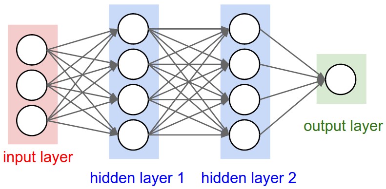
Left: A regular 3-layer Neural Network. Right: A ConvNet arranges its neurons in three dimensions (width, height, depth), as visualized in one of the layers. Every layer of a ConvNet transforms the 3D input volume to a 3D output volume of neuron activations. In this example, the red input layer holds the image, so its width and height would be the dimensions of the image, and the depth would be 3 (Red, Green, Blue channels).
A ConvNet is made up of Layers. Every Layer has a simple API: It transforms an input 3D volume to an output 3D volume with some differentiable function that may or may not have parameters.
ConvNet Layers
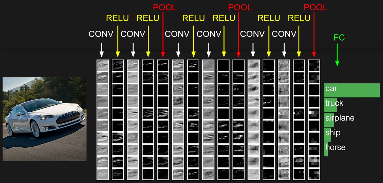
Example Architecture: Overview. We will go into more details below, but a simple ConvNet for CIFAR-10 classification could have the architecture [INPUT - CONV - RELU - POOL - FC]. In more detail:
- INPUT [32x32x3] will hold the raw pixel values of the image, in this case an image of width 32, height 32, and with three color channels R,G,B.
- CONV layer will compute the output of neurons that are connected to local regions in the input, each computing a dot product between their weights and a small region they are connected to in the input volume. This may result in volume such as [32x32x12] if we decided to use 12 filters.
- RELU layer will apply an elementwise activation function, such as the max(0,x) thresholding at zero. This leaves the size of the volume unchanged ([32x32x12]).
- POOL layer will perform a downsampling operation along the spatial dimensions (width, height), resulting in volume such as [16x16x12].
- FC (i.e. fully-connected) layer will compute the class scores, resulting in volume of size [1x1x10], where each of the 10 numbers correspond to a class score, such as among the 10 categories of CIFAR-10. As with ordinary Neural Networks and as the name implies, each neuron in this layer will be connected to all the numbers in the previous volume.
In this way, ConvNets transform the original image layer by layer from the original pixel values to the final class scores. Note that some layers contain parameters and other don’t. In particular, the CONV/FC layers perform transformations that are a function of not only the activations in the input volume, but also of the parameters (the weights and biases of the neurons). On the other hand, the RELU/POOL layers will implement a fixed function. The parameters in the CONV/FC layers will be trained with gradient descent so that the class scores that the ConvNet computes are consistent with the labels in the training set for each image.
We now describe the individual layers and the details of their hyperparameters and their connectivities.
Convolutional Layer
- Local Connectivity. When dealing with high-dimensional inputs such as images, as we saw above it is impractical to connect neurons to all neurons in the previous volume. Instead, we will connect each neuron to only a local region of the input volume. The spatial extent of this connectivity is a hyperparameter called the receptive field of the neuron (equivalently this is the filter size). The extent of the connectivity along the depth axis is always equal to the depth of the input volume.
Example 1. For example, suppose that the input volume has size [32x32x3], (e.g. an RGB CIFAR-10 image). If the receptive field (or the filter size) is 5x5, then each neuron in the Conv Layer will have weights to a [5x5x3] region in the input volume, for a total of 5 * 5 * 3 = 75 weights (and +1 bias parameter). Notice that the extent of the connectivity along the depth axis must be 3, since this is the depth of the input volume.
Example 2. Suppose an input volume had size [16x16x20]. Then using an example receptive field size of 3x3, every neuron in the Conv Layer would now have a total of 3 * 3 * 20 = 180 connections to the input volume. Notice that, again, the connectivity is local in space (e.g. 3x3), but full along the input depth (20).
- Spatial arrangement. Three hyperparameters control the size of the output volume: the depth, stride and zero-padding. We discuss these next:
First, the depth of the output volume is a hyperparameter: it corresponds to the number of filters we would like to use, each learning to look for something different in the input. For example, if the first Convolutional Layer takes as input the raw image, then different neurons along the depth dimension may activate in presence of various oriented edged, or blobs of color. We will refer to a set of neurons that are all looking at the same region of the input as a depth column (some people also prefer the term fibre).
Pooling Layer
Its function is to progressively reduce the spatial size of the representation to reduce the amount of parameters and computation in the network, and hence to also control overfitting.
The Pooling Layer operates independently on every depth slice of the input and resizes it spatially, using the MAX operation. The most common form is a pooling layer with filters of size 2x2 applied with a stride of 2 downsamples every depth slice in the input by 2 along both width and height, discarding 75% of the activations.
- Getting rid of pooling. Many people dislike the pooling operation and think that we can get away without it. For example, Striving for Simplicity: The All Convolutional Net proposes to discard the pooling layer in favor of architecture that only consists of repeated CONV layers. To reduce the size of the representation they suggest using larger stride in CONV layer once in a while. Discarding pooling layers has also been found to be important in training good generative models, such as variational autoencoders (VAEs) or generative adversarial networks (GANs). It seems likely that future architectures will feature very few to no pooling layers.
Normalization Layer
In practice their contribution has been shown to be minimal, if any. For various types of normalizations, see the discussion in Alex Krizhevsky’s cuda-convnet library API.
Converting Fully-Connected Layers to Convolutional Layers
It is worth noting that the only difference between FC and CONV layers is that the neurons in the CONV layer are connected only to a local region in the input, and that many of the neurons in a CONV volume share parameters.
Consider a ConvNet architecture that takes a 224x224x3 image, and then uses a series of CONV layers and POOL layers to reduce the image to an activations volume of size 7x7x512 (in an AlexNet architecture that we’ll see later, this is done by use of 5 pooling layers that downsample the input spatially by a factor of two each time, making the final spatial size 224/2/2/2/2/2 = 7).
ConvNet Architectures
In this section we discuss how these are commonly stacked together to form entire ConvNets.
Layer Patterns
INPUT -> [CONV -> RELU -> POOL]*2 -> FC -> RELU -> FC. Here we see that there is a single CONV layer between every POOL layer.INPUT -> [CONV -> RELU -> CONV -> RELU -> POOL]*3 -> [FC -> RELU]*2 -> FCHere we see two CONV layers stacked before every POOL layer. This is generally a good idea for larger and deeper networks, because multiple stacked CONV layers can develop more complex features of the input volume before the destructive pooling operation.
Prefer a stack of small filter CONV to one large receptive field CONV layer.
Suppose that you stack three 3x3 CONV layers on top of each other (with non-linearities in between, of course). In this arrangement, each neuron on the first CONV layer has a 3x3 view of the input volume. A neuron on the second CONV layer has a 3x3 view of the first CONV layer, and hence by extension a 5x5 view of the input volume. Similarly, a neuron on the third CONV layer has a 3x3 view of the 2nd CONV layer, and hence a 7x7 view of the input volume. Suppose that instead of these three layers of 3x3 CONV, we only wanted to use a single CONV layer with 7x7 receptive fields. These neurons would have a receptive field size of the input volume that is identical in spatial extent (7x7), but with several disadvantages. First, the neurons would be computing a linear function over the input, while the three stacks of CONV layers contain non-linearities that make their features more expressive. Second, if we suppose that all the volumes have C
C channels, then it can be seen that the single 7x7 CONV layer would contain 49^2 * C parameters, while the three 3x3 CONV layers would only contain 3×(C×(3×3×C))=27 * C^2 parameters. Intuitively, stacking CONV layers with tiny filters as opposed to having one CONV layer with big filters allows us to express more powerful features of the input, and with fewer parameters. As a practical disadvantage, we might need more memory to hold all the intermediate CONV layer results if we plan to do backpropagation.
Layer Sizing Patterns
The input layer (that contains the image) should be divisible by 2 many times. Common numbers include 32 (e.g. CIFAR-10), 64, 96 (e.g. STL-10), or 224 (e.g. common ImageNet ConvNets), 384, and 512.
The conv layers should be using small filters (e.g. 3x3 or at most 5x5), using a stride of S=1, and crucially, padding the input volume with zeros in such way that the conv layer does not alter the spatial dimensions of the input.
The pool layers are in charge of downsampling the spatial dimensions of the input. The most common setting is to use max-pooling with 2x2 receptive fields.
Reducing sizing headaches. The scheme presented above is pleasing because all the CONV layers preserve the spatial size of their input, while the POOL layers alone are in charge of down-sampling the volumes spatially. In an alternative scheme where we use strides greater than 1 or don’t zero-pad the input in CONV layers, we would have to very carefully keep track of the input volumes throughout the CNN architecture and make sure that all strides and filters “work out”, and that the ConvNet architecture is nicely and symmetrically wired.
Why use stride of 1 in CONV? Smaller strides work better in practice. Additionally, as already mentioned stride 1 allows us to leave all spatial down-sampling to the POOL layers, with the CONV layers only transforming the input volume depth-wise.
Why use padding? In addition to the aforementioned benefit of keeping the spatial sizes constant after CONV, doing this actually improves performance. If the CONV layers were to not zero-pad the inputs and only perform valid convolutions, then the size of the volumes would reduce by a small amount after each CONV, and the information at the borders would be “washed away” too quickly.
Compromising based on memory constraints. In some cases (especially early in the ConvNet architectures), the amount of memory can build up very quickly with the rules of thumb presented above. For example, filtering a 224x224x3 image with three 3x3 CONV layers with 64 filters each and padding 1 would create three activation volumes of size [224x224x64]. This amounts to a total of about 10 million activations, or 72MB of memory (per image, for both activations and gradients). Since GPUs are often bottlenecked by memory, it may be necessary to compromise. In practice, people prefer to make the compromise at only the first CONV layer of the network. For example, one compromise might be to use a first CONV layer with filter sizes of 7x7 and stride of 2 (as seen in a ZF net). As another example, an AlexNet uses filter sizes of 11x11 and stride of 4.
Case Studies (LeNet / AlexNet / ZFNet / GoogLeNet / VGGNet)
There are several architectures in the field of Convolutional Networks that have a name. The most common are:
- LeNet. The first successful applications of Convolutional Networks were developed by Yann LeCun in 1990’s. Of these, the best known is the LeNet architecture that was used to read zip codes, digits, etc.
- AlexNet. The first work that popularized Convolutional Networks in Computer Vision was the AlexNet, developed by Alex Krizhevsky, Ilya Sutskever and Geoff Hinton. The AlexNet was submitted to the ImageNet ILSVRC challenge in 2012 and significantly outperformed the second runner-up (top 5 error of 16% compared to runner-up with 26% error). The Network had a very similar architecture to LeNet, but was deeper, bigger, and featured Convolutional Layers stacked on top of each other (previously it was common to only have a single CONV layer always immediately followed by a POOL layer).
- ZF Net. The ILSVRC 2013 winner was a Convolutional Network from Matthew Zeiler and Rob Fergus. It became known as the ZFNet (short for Zeiler & Fergus Net). It was an improvement on AlexNet by tweaking the architecture hyperparameters, in particular by expanding the size of the middle convolutional layers and making the stride and filter size on the first layer smaller.
- GoogLeNet. The ILSVRC 2014 winner was a Convolutional Network from Szegedy et al. from Google. Its main contribution was the development of an Inception Module that dramatically reduced the number of parameters in the network (4M, compared to AlexNet with 60M). Additionally, this paper uses Average Pooling instead of Fully Connected layers at the top of the ConvNet, eliminating a large amount of parameters that do not seem to matter much. There are also several followup versions to the GoogLeNet, most recently Inception-v4.
- VGGNet. The runner-up in ILSVRC 2014 was the network from Karen Simonyan and Andrew Zisserman that became known as the VGGNet. Its main contribution was in showing that the depth of the network is a critical component for good performance. Their final best network contains 16 CONV/FC layers and, appealingly, features an extremely homogeneous architecture that only performs 3x3 convolutions and 2x2 pooling from the beginning to the end. Their pretrained model is available for plug and play use in Caffe. A downside of the VGGNet is that it is more expensive to evaluate and uses a lot more memory and parameters (140M). Most of these parameters are in the first fully connected layer, and it was since found that these FC layers can be removed with no performance downgrade, significantly reducing the number of necessary parameters.
- ResNet. Residual Network developed by Kaiming He et al. was the winner of ILSVRC 2015. It features special skip connections and a heavy use of batch normalization. The architecture is also missing fully connected layers at the end of the network. The reader is also referred to Kaiming’s presentation (video, slides), and some recent experiments that reproduce these networks in Torch. ResNets are currently by far state of the art Convolutional Neural Network models and are the default choice for using ConvNets in practice (as of May 10, 2016). In particular, also see more recent developments that tweak the original architecture from Kaiming He et al. Identity Mappings in Deep Residual Networks (published March 2016).
Computational Considerations
The largest bottleneck to be aware of when constructing ConvNet architectures is the memory bottleneck. Many modern GPUs have a limit of 3/4/6GB memory, with the best GPUs having about 12GB of memory. There are three major sources of memory to keep track of:
-
From the intermediate volume sizes: These are the raw number of activations at every layer of the ConvNet, and also their gradients (of equal size). Usually, most of the activations are on the earlier layers of a ConvNet (i.e. first Conv Layers). These are kept around because they are needed for backpropagation, but a clever implementation that runs a ConvNet only at test time could in principle reduce this by a huge amount, by only storing the current activations at any layer and discarding the previous activations on layers below.
-
From the parameter sizes: These are the numbers that hold the network parameters, their gradients during backpropagation, and commonly also a step cache if the optimization is using momentum, Adagrad, or RMSProp. Therefore, the memory to store the parameter vector alone must usually be multiplied by a factor of at least 3 or so.
-
Every ConvNet implementation has to maintain miscellaneous memory, such as the image data batches, perhaps their augmented versions, etc.
Once you have a rough estimate of the total number of values (for activations, gradients, and misc), the number should be converted to size in GB. Take the number of values, multiply by 4 to get the raw number of bytes (since every floating point is 4 bytes, or maybe by 8 for double precision), and then divide by 1024 multiple times to get the amount of memory in KB, MB, and finally GB. If your network doesn’t fit, a common heuristic to “make it fit” is to decrease the batch size, since most of the memory is usually consumed by the activations.
Additional References
See the original website