Cs231n Optimization Sgd

Optimization is the process of finding the set of parameters W that minimize the loss function.

Visualizing the loss function

The full SVM loss (without regularization) becomes:

\begin{aligned} L_{0} = & max (0, w_{1}^{T} x_{0} - w_{0}^{T} x_{0} + 1) + max (0, w_{2}^{T} x_{0} - w_{0}^{T} x_{0} + 1) \\ L_{1} = & max (0, w_{0}^{T} x_{1} - w_{1}^{T} x_{1} + 1) + max (0, w_{2}^{T} x_{1} - w_{1}^{T} x_{1} + 1) \\ L_{2} = & max (0, w_{0}^{T} x_{2} - w_{2}^{T} x_{2} + 1) + max (0, w_{1}^{T} x_{2} - w_{2}^{T} x_{2} + 1) \\ L = & (L_{0} + L_{1} + L_{2}) / 3 \end{aligned}

svmbowl

Once we extend our score functions f to Neural Networks our objective functions will become non-convex, and the visualizations above will not feature bowls but complex, bumpy terrains.

Non-differentiable loss functions. As a technical note, you can also see that the kinks in the loss function (due to the max operation) technically make the loss function non-differentiable because at these kinks the gradient is not defined. However, the subgradient still exists and is commonly used instead. In this class will use the terms subgradient 次梯度 and gradient interchangeably.

Optimization

Strategy 1: A first very bad idea solution: Random Search

numpy.random.randn(d0, d1, ..., dn)
Return a sample (or samples) from the “standard normal” distribution.

Parameters:	
d0, d1, ..., dn : int, optional
The dimensions of the returned array, should be all positive. If no argument is given a single Python float is returned.

Our strategy will be to start with random weights and iteratively refine them over time to get lower loss

Strategy #2: Random Local Search

Concretely, we will start out with a random W, generate random perturbations δW to it and if the loss at the perturbed W+δW is lower, we will perform an update. The code for this procedure is as follows:

 W = np.random.randn(10, 3073) * 0.001 # generate random starting W
bestloss = float("inf")
for i in xrange(1000):
  step_size = 0.0001
  Wtry = W + np.random.randn(10, 3073) * step_size
  loss = L(Xtr_cols, Ytr, Wtry)
  if loss < bestloss:
    W = Wtry
    bestloss = loss
  print 'iter %d loss is %f' % (i, bestloss)

Strategy #3: Following the gradient

In the previous section we tried to find a direction in the weight-space that would improve our weight vector (and give us a lower loss). It turns out that there is no need to randomly search for a good direction: we can compute the best direction along which we should change our weight vector that is mathematically guaranteed to be the direction of the steepest descend (at least in the limit as the step size goes towards zero). This direction will be related to the gradient of the loss function.

The mathematical expression for the derivative of a 1-D function with respect its input is:

\frac{df(x)}{dx} = \lim_{h\ \to 0} \frac{f(x + h) - f(x)}{h}

When the functions of interest take a vector of numbers instead of a single number, we call the derivatives partial derivatives, and the gradient is simply the vector of partial derivatives in each dimension.

Computing the gradient

There are two ways to compute the gradient: A slow, approximate but easy way (numerical gradient), and a fast, exact but more error-prone way that requires calculus (analytic gradient). We will now present both.

Numerically with finite differences

The gradient tells us the slope of the loss function along every dimension, which we can use to make an update:

loss_original = CIFAR10_loss_fun(W) # the original loss
print 'original loss: %f' % (loss_original, )

# lets see the effect of multiple step sizes
for step_size_log in [-10, -9, -8, -7, -6, -5,-4,-3,-2,-1]:
  step_size = 10 ** step_size_log
  W_new = W - step_size * df # new position in the weight space
  loss_new = CIFAR10_loss_fun(W_new)
  print 'for step size %f new loss: %f' % (step_size, loss_new)
  
  # prints:
# original loss: 2.200718
# for step size 1.000000e-10 new loss: 2.200652
# for step size 1.000000e-09 new loss: 2.200057
# for step size 1.000000e-08 new loss: 2.194116
# for step size 1.000000e-07 new loss: 2.135493
## chose！ for step size 1.000000e-06 new loss: 1.647802
# for step size 1.000000e-05 new loss: 2.844355

step size !!!! matters !

Update in negative gradient direction. In the code above, notice that to compute W_new we are making an update in the negative direction of the gradient df since we wish our loss function to decrease, not increase.

Analytically with calculus

The above method is very computationally expensive to compute. The second way to compute the gradient is analytically using Calculus, which allows us to derive a direct formula for the gradient (no approximations) that is also very fast to compute. However, unlike the numerical gradient it can be more error prone to implement, which is why in practice it is very common to compute the analytic gradient and compare it to the numerical gradient to check the correctness of your implementation. This is called a gradient check.

We can differentiate the function with respect to the weights. For example, taking the gradient with respect to wyi we obtain:

\nabla_{w_{y_{i}}} L_{i} = - (\sum_{j \neq y_{i}} 1 (w_{j}^{T} x_{i} - w_{y_{i}}^{T} x_{i} + Δ > 0)) x_{i}

Gradient descent

Now that we can compute the gradient of the loss function, the procedure of repeatedly evaluating the gradient and then performing a parameter update is called Gradient Descent. Its vanilla version looks as follows:

# Vanilla Gradient Descent

while True:
  weights_grad = evaluate_gradient(loss_fun, data, weights)
  weights += - step_size * weights_grad # perform parameter update

This simple loop is at the core of all Neural Network libraries. There are other ways of performing the optimization (e.g. LBFGS), but Gradient Descent is currently by far the most common and established way of optimizing Neural Network loss functions. Throughout the class we will put some bells and whistles on the details of this loop (e.g. the exact details of the update equation), but the core idea of following the gradient until we’re happy with the results will remain the same.

Mini-batch gradient descent. In large-scale applications (such as the ILSVRC challenge), the training data can have on order of millions of examples. Hence, it seems wasteful to compute the full loss function over the entire training set in order to perform only a single parameter update. A very common approach to addressing this challenge is to compute the gradient over batches of the training data. For example, in current state of the art ConvNets, a typical batch contains 256 examples from the entire training set of 1.2 million. This batch is then used to perform a parameter update:

# Vanilla Minibatch Gradient Descent

while True:
  data_batch = sample_training_data(data, 256) # sample 256 examples
  weights_grad = evaluate_gradient(loss_fun, data_batch, weights)
  weights += - step_size * weights_grad # perform parameter update

when we average the data loss over all 1.2 million images we would get the exact same loss as if we only evaluated on a small subset of 1000. In practice of course, the dataset would not contain duplicate images, the gradient from a mini-batch is a good approximation of the gradient of the full objective. Therefore, much faster convergence can be achieved in practice by evaluating the mini-batch gradients to perform more frequent parameter updates.

The extreme case of this is a setting where the mini-batch contains only a single example. This process is called Stochastic Gradient Descent (SGD) (or also sometimes on-line gradient descent).

The size of the mini-batch is a hyperparameter but it is not very common to cross-validate it. It is usually based on memory constraints (if any), or set to some value, e.g. 32, 64 or 128. We use powers of 2 in practice because many vectorized operation implementations work faster when their inputs are sized in powers of 2.

Summary

dataflow

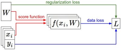
Summary of the information flow. The dataset of pairs of (x,y) is given and fixed. The weights start out as random numbers and can change. During the forward pass the score function computes class scores, stored in vector f. The loss function contains two components: The data loss computes the compatibility between the scores f and the labels y. The regularization loss is only a function of the weights. During Gradient Descent, we compute the gradient on the weights (and optionally on data if we wish) and use them to perform a parameter update during Gradient Descent.

In this section,

We developed the intuition of the loss function as a high-dimensional optimization landscape in which we are trying to reach the bottom. The working analogy we developed was that of a blindfolded hiker who wishes to reach the bottom. In particular, we saw that the SVM cost function is piece-wise linear and bowl-shaped.
We motivated the idea of optimizing the loss function with iterative refinement, where we start with a random set of weights and refine them step by step until the loss is minimized.
We saw that the gradient of a function gives the steepest ascent direction and we discussed a simple but inefficient way of computing it numerically using the finite difference approximation (the finite difference being the value of h used in computing the numerical gradient).
We saw that the parameter update requires a tricky setting of the step size (or the learning rate) that must be set just right: if it is too low the progress is steady but slow. If it is too high the progress can be faster, but more risky. We will explore this tradeoff in much more detail in future sections.
We discussed the tradeoffs between computing the numerical and analytic gradient. The numerical gradient is simple but it is approximate and expensive to compute. The analytic gradient is exact, fast to compute but more error-prone since it requires the derivation of the gradient with math. Hence, in practice we always use the analytic gradient and then perform a gradient check, in which its implementation is compared to the numerical gradient.
We introduced the Gradient Descent algorithm which iteratively computes the gradient and performs a parameter update in loop.

Coming up: The core takeaway from this section is that the ability to compute the gradient of a loss function with respect to its weights (and have some intuitive understanding of it) is the most important skill needed to design, train and understand neural networks. In the next section we will develop proficiency in computing the gradient analytically using the chain rule, otherwise also referred to as backpropagation. This will allow us to efficiently optimize relatively arbitrary loss functions that express all kinds of Neural Networks, including Convolutional Neural Networks.