Cs231n Linear Classification
The approach will have two major components: a score function that maps the raw data to class scores, and a loss function that quantifies the agreement between the predicted scores and the ground truth labels.
As we saw, kNN has a number of disadvantages:
- The classifier must remember all of the training data and store it for future comparisons with the test data. This is space inefficient because datasets may easily be gigabytes in size.
- Classifying a test image is expensive since it requires a comparison to all training images.
Intro to Linear classification
Parameterized mapping from images to label scores
Linear classifier. In this module we will start out with arguably the simplest possible function, a linear mapping:
- An advantage of this approach is that the training data is used to learn the parameters W,b, but once the learning is complete we can discard the entire training set and only keep the learned parameters. That is because a new test image can be simply forwarded through the function and classified based on the computed scores.
As we saw above, every row of W is a classifier for one of the classes. The geometric interpretation of these numbers is that as we change one of the rows of W, the corresponding line in the pixel space will rotate in different directions. The biases b, on the other hand, allow our classifiers to translate the lines. In particular, note that without the bias terms, plugging in xi=0 would always give score of zero regardless of the weights, so all lines would be forced to cross the origin.
Interpretation of linear classifiers as template matching. Another interpretation for the weights Wis that each row of W corresponds to a template (or sometimes also called a prototype) for one of the classes. The score of each class for an image is then obtained by comparing each template with the image using an inner product (or dot product) one by one to find the one that “fits” best. With this terminology, the linear classifier is doing template matching, where the templates are learned. Another way to think of it is that we are still effectively doing Nearest Neighbor, but instead of having thousands of training images we are only using a single image per class (although we will learn it, and it does not necessarily have to be one of the images in the training set), and we use the (negative) inner product as the distance instead of the L1 or L2 distance.
Bias trick. Before moving on we want to mention a common simplifying trick to representing the two parameters W,b
as one. Recall that we defined the score function as: f(xi,W,b)=Wxi+b
As we proceed through the material it is a little cumbersome to keep track of two sets of parameters (the biases b and weights W separately. A commonly used trick is to combine the two sets of parameters into a single matrix that holds both of them by extending the vector xi with one additional dimension that always holds the constant 1 - a default bias dimension. With the extra dimension, the new score function will simplify to a single matrix multiply: f(xi,W)=Wxi
With our CIFAR-10 example, xi is now [3073 x 1] instead of [3072 x 1] - (with the extra dimension holding the constant 1), and W
is now [10 x 3073] instead of [10 x 3072]. The extra column that W now corresponds to the bias b. An illustration might help clarify:

Image data preprocessing. The raw pixel values (which range from [0…255]), common preprocessing is to scale each input feature so that its values range from [-1, 1].
Loss function
Intuitively, the loss will be high if we’re doing a poor job of classifying the training data, and it will be low if we’re doing well.
Multiclass SVM
Let’s now get more precise. Recall that for the i-th example we are given the pixels of image xi and the label yi that specifies the index of the correct class. The score function takes the pixels and computes the vector f(xi,W) of class scores, which we will abbreviate to s s (short for scores). For example, the score for the j-th class is the j-th element:
</math> Example. Lets unpack this with an example to see how it works. Suppose that we have three classes that receive the scores
, and that the first class is the true class (i.e.
</math>. Also assume that
</math> (a hyperparameter we will go into more detail about soon) is 10. The expression above sums over all incorrect classes (j≠yi), so we get two terms:
You can see that the first term gives zero since [-7 - 13 + 10] gives a negative number, which is then thresholded to zero with the max(0,−) function. We get zero loss for this pair because the correct class score (13) was greater than the incorrect class score (-7) by at least the margin 10. In fact the difference was 20, which is much greater than 10 but the SVM only cares that the difference is at least 10; Any additional difference above the margin is clamped at zero with the max operation. The second term computes [11 - 13 + 10] which gives 8. That is, even though the correct class had a higher score than the incorrect class (13 > 11), it was not greater by the desired margin of 10. The difference was only 2, which is why the loss comes out to 8 (i.e. how much higher the difference would have to be to meet the margin). In summary, the SVM loss function wants the score of the correct class yi to be larger than the incorrect class scores by at least by Δ (delta). If this is not the case, we will accumulate loss.
The loss function quantifies our unhappiness with predictions on the training set
Regularization.
Notice that the regularization function is not a function of the data, it is only based on the weights. Including the regularization penalty completes the full Multiclass Support Vector Machine loss, which is made up of two components: the data loss (which is the average loss Li over all examples) and the regularization loss.
Practical Considerations
The hyperparameters Δ and λ seem like two different hyperparameters, but in fact they both control the same tradeoff: The tradeoff between the data loss and the regularization loss in the objective.
Softmax classifier
It turns out that the SVM is one of two commonly seen classifiers. The other popular choice is the Softmax classifier, which has a different loss function. If you’ve heard of the binary Logistic Regression classifier before, the Softmax classifier is its generalization to multiple classes.
Softmax classifier gives a slightly more intuitive output (normalized class probabilities)
where we are using the notation fj to mean the j-th element of the vector of class scores f.
SVM vs Softmax
A picture might help clarify the distinction between the Softmax and SVM classifiers:
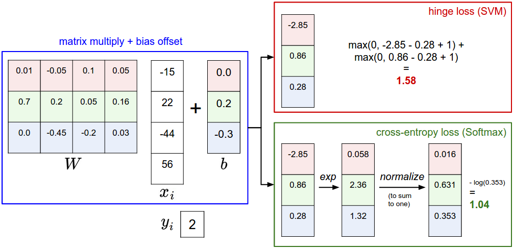
Example of the difference between the SVM and Softmax classifiers for one datapoint. In both cases we compute the same score vector f (e.g. by matrix multiplication in this section). The difference is in the interpretation of the scores in f: The SVM interprets these as class scores and its loss function encourages the correct class (class 2, in blue) to have a score higher by a margin than the other class scores. The Softmax classifier instead interprets the scores as (unnormalized) log probabilities for each class and then encourages the (normalized) log probability of the correct class to be high (equivalently the negative of it to be low). The final loss for this example is 1.58 for the SVM and 1.04 (note this is 1.04 using the natural logarithm, not base 2 or base 10) for the Softmax classifier, but note that these numbers are not comparable; They are only meaningful in relation to loss computed within the same classifier and with the same data.
Softmax classifier provides “probabilities” for each class. Unlike the SVM which computes uncalibrated and not easy to interpret scores for all classes, the Softmax classifier allows us to compute “probabilities” for all labels. For example, given an image the SVM classifier might give you scores [12.5, 0.6, -23.0] for the classes “cat”, “dog” and “ship”. The softmax classifier can instead compute the probabilities of the three labels as [0.9, 0.09, 0.01], which allows you to interpret its confidence in each class.
Summary
In summary,
We defined a score function from image pixels to class scores (in this section, a linear function that depends on weights W and biases b).
-
Unlike kNN classifier, the advantage of this parametric approach is that once we learn the parameters we can discard the training data. Additionally, the prediction for a new test image is fast since it requires a single matrix multiplication with W, not an exhaustive comparison to every single training example.
-
We introduced the bias trick, which allows us to fold the bias vector into the weight matrix for convenience of only having to keep track of one parameter matrix.
-
We defined a loss function (we introduced two commonly used losses for linear classifiers: the SVM and the Softmax) that measures how compatible a given set of parameters is with respect to the ground truth labels in the training dataset. We also saw that the loss function was defined in such way that making good predictions on the training data is equivalent to having a small loss.
We now saw one way to take a dataset of images and map each one to class scores based on a set of parameters, and we saw two examples of loss functions that we can use to measure the quality of the predictions.
But how do we efficiently determine the parameters that give the best (lowest) loss? This process is optimization, and it is the topic of the next section.