Cs231n Backpropagation
Motivation. In this section we will develop expertise with an intuitive understanding of backpropagation, which is a way of computing gradients of expressions through recursive application of chain rule. Understanding of this process and its subtleties is critical for you to understand, and effectively develop, design and debug Neural Networks.
Problem statement. The core problem studied in this section is as follows: We are given some function f(x) is a vector of inputs and we are interested in computing the gradient of f at x (i.e. ∇f(x) ).
Simple expressions and interpretation of the gradient
The derivative on each variable tells you the sensitivity of the whole expression on its value.
Compound expressions with chain rule
The chain rule tells us that the correct way to “chain” these gradient expressions together is through multiplication. For example,
</math>. In practice this is simply a multiplication of the two numbers that hold the two gradients.
Intuitive understanding of backpropagation
This extra multiplication (for each input) due to the chain rule can turn a single and relatively useless gate into a cog in a complex circuit such as an entire neural network.
-
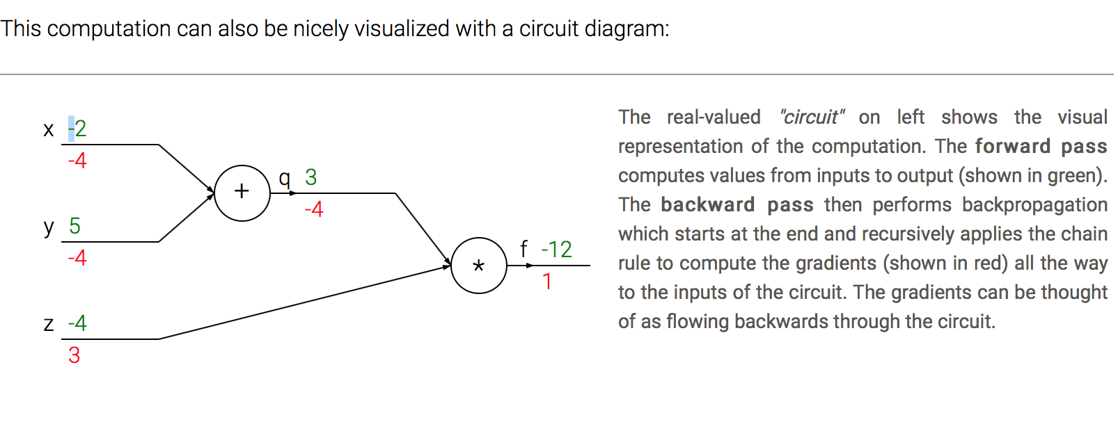
Lets get an intuition for how this works by referring again to the example. The add gate received inputs [-2, 5] and computed output 3. Since the gate is computing the addition operation, its local gradient for both of its inputs is +1. The rest of the circuit computed the final value, which is -12.
-
During the backward pass in which the chain rule is applied recursively backwards through the circuit, the add gate (which is an input to the multiply gate) learns that the gradient for its output was -4. If we anthropomorphize the circuit as wanting to output a higher value (which can help with intuition), then we can think of the circuit as “wanting” the output of the add gate to be lower (due to negative sign), and with a force of 4.
-
To continue the recurrence and to chain the gradient, the add gate takes that gradient and multiplies it to all of the local gradients for its inputs (making the gradient on both x and y 1 * -4 = -4). Notice that this has the desired effect: If x,y were to decrease (responding to their negative gradient) then the add gate’s output would decrease, which in turn makes the multiply gate’s output increase.
Backpropagation can thus be thought of as gates communicating to each other (through the gradient signal) whether they want their outputs to increase or decrease (and how strongly), so as to make the final output value higher.
Modularity: Sigmoid example
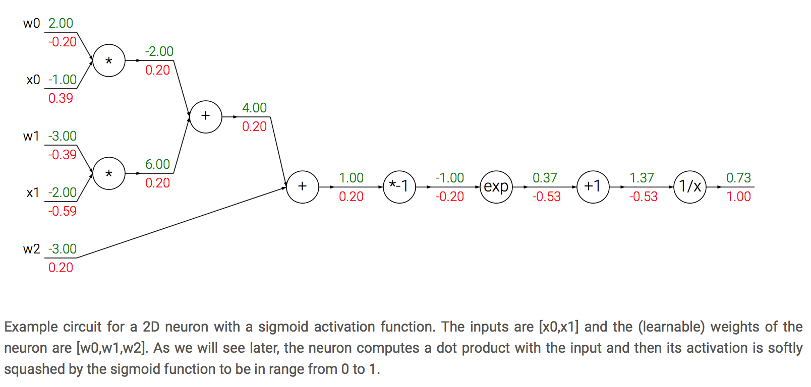
Cache forward pass variables. To compute the backward pass it is very helpful to have some of the variables that were used in the forward pass. In practice you want to structure your code so that you cache these variables, and so that they are available during backpropagation. If this is too difficult, it is possible (but wasteful) to recompute them.
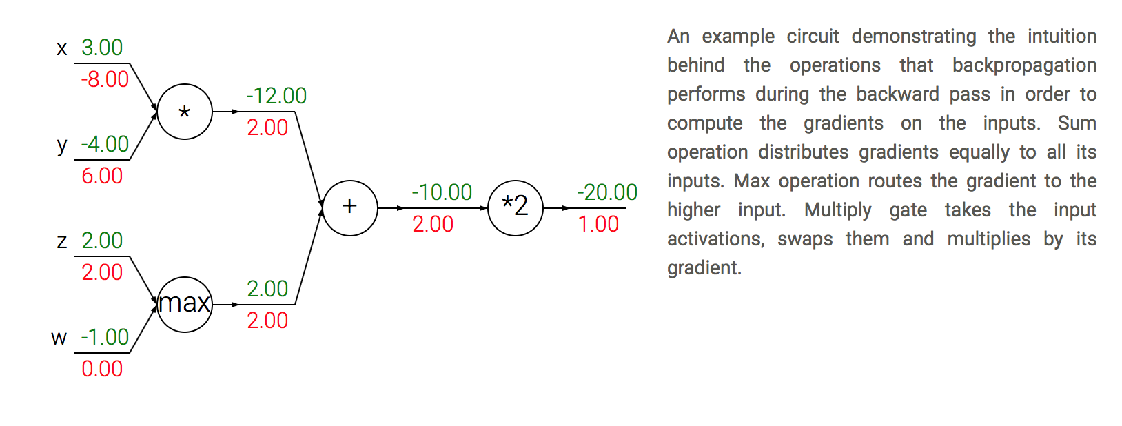
Patterns in backward flow
Gradients for vectorized operations
The above sections were concerned with single variables, but all concepts extend in a straight-forward manner to matrix and vector operations. However, one must pay closer attention to dimensions and transpose operations.
Matrix-Matrix multiply gradient. Possibly the most tricky operation is the matrix-matrix multiplication (which generalizes all matrix-vector and vector-vector) multiply operations:
# forward pass
W = np.random.randn(5, 10)
X = np.random.randn(10, 3)
D = W.dot(X)

# now suppose we had the gradient on D from above in the circuit
dD = np.random.randn(*D.shape) # same shape as D
dW = dD.dot(X.T) #.T gives the transpose of the matrix
dX = W.T.dot(dD)
Summary
- We developed intuition for what the gradients mean, how they flow backwards in the circuit, and how they communicate which part of the circuit should increase or decrease and with what force to make the final output higher.
-
We discussed the importance of staged computation for practical implementations of backpropagation. You always want to break up your function into modules for which you can easily derive local gradients, and then chain them with chain rule.
- Crucially, you almost never want to write out these expressions on paper and differentiate them symbolically in full, because you never need an explicit mathematical equation for the gradient of the input variables. Hence, decompose your expressions into stages such that you can differentiate every stage independently (the stages will be matrix vector multiplies, or max operations, or sum operations, etc.) and then backprop through the variables one step at a time.
In the next section we will start to define Neural Networks, and backpropagation will allow us to efficiently compute the gradients on the connections of the neural network, with respect to a loss function. In other words, we’re now ready to train Neural Nets, and the most conceptually difficult part of this class is behind us! ConvNets will then be a small step away.