Intro Distributed Deep Learning
We’ll look at how the training of deep learning models can be significantly accelerated with distributed computing on GPUs, as well as discuss some of the challenges and examine current research on the topic. The original post is here, the reason I re-copy the post is that it’s and my equations both do not render properly in browser because…
But you can download or find the proper disply is here!!
Nothing can stop us, right?!
[toc]
Introduction
Training these neural network models is computationally demanding. Although in recent years significant advances have been made in GPU hardware, network architectures and training methods, the fact remains that network training can take an impractically long time on a single machine. Fortunately, we are not restricted to a single machine: a significant amount of work and research has been conducted on enabling the efficient distributed training of neural networks.
We’ll start by considering two approaches to parallelizing/distributing our training computation.
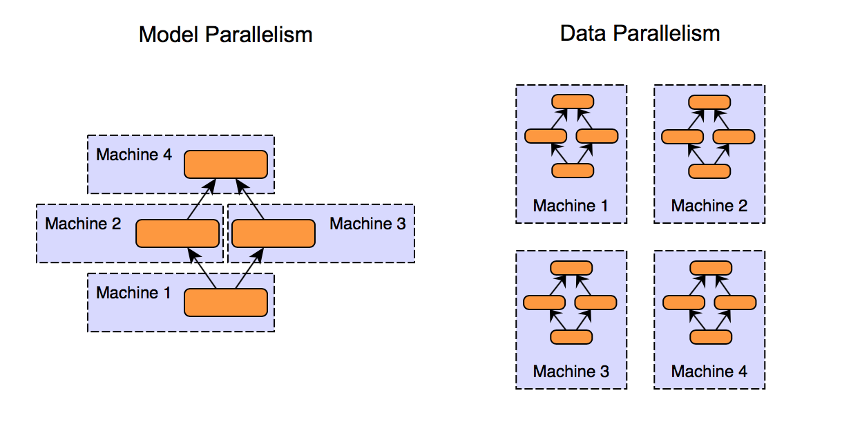
In model parallelism, different machines in the distributed system are responsible for the computations in different parts of a single network - for example, each layer in the neural network may be assigned to a different machine.
In data parallelism, different machines have a complete copy of the model; each machine simply gets a different portion of the data, and results from each are somehow combined.
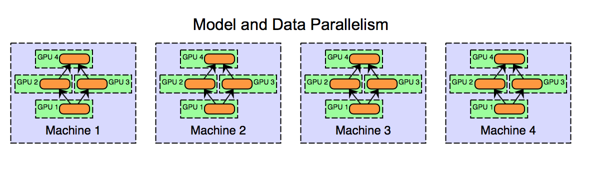
Of course, these approaches are not mutually exclusive. Consider a cluster of multi-GPU systems. We could use model parallelism (model split across GPUs) for each machine, and data parallelism between machines.
While model parallelism can work well in practice, data parallelism is arguably the preferred approach for distributed systems and has been the focus of more research. For one thing, implementation, fault tolerance and good cluster utilization is easier for data parallelism than for model parallelism. Model parallelism in the context of distributed systems is interesting and does have some benefits (such as scalability to large models), but here we will be focusing on data parallelism.
Data Parallelism
Data parallel approaches to distributed training keep a copy of the entire model on each worker machine, processing different subsets of the training data set on each. Data parallel training approaches all require some method of combining results and synchronizing the model parameters between each worker. A number of different approaches have been discussed in the literature, and the primary differences between approaches are
- Parameter averaging vs. update (gradient)-based approaches
- Synchronous vs. asynchronous methods
- Centralized vs. distributed synchronization
Deeplearning4j’s current Spark implementation is a synchronous parameter averaging where the Spark driver and reduction operations take the place of a parameter server.
Parameter Averaging
Parameter averaging is the conceptually simplest approach to data parallelism. With parameter averaging, training proceeds as follows:
- Initialize the network parameters randomly based on the model configuration
- Distribute a copy of the current parameters to each worker
- Train each worker on a subset of the data
- Set the global parameters to the average the parameters from each worker
- While there is more data to process, go to step 2
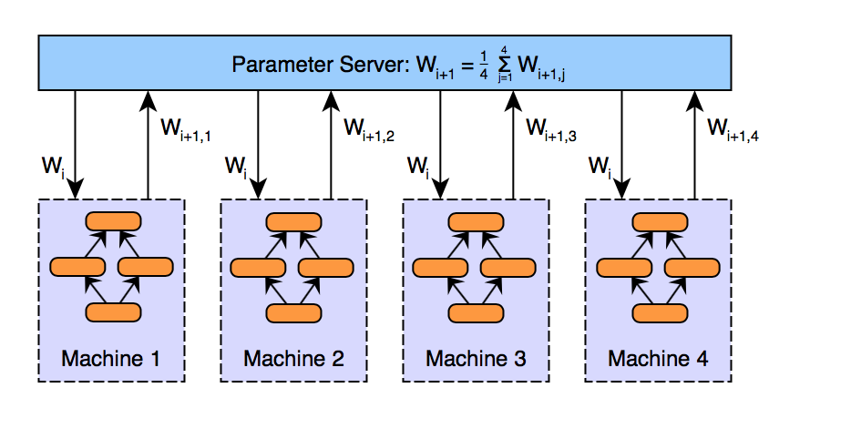
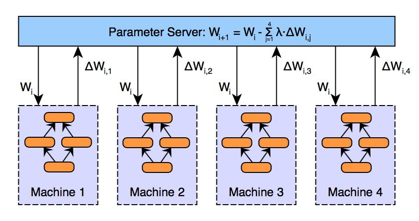
Steps 2 through 4 are demonstrated in the image below. In this diagram, W represents the parameters (weights, biases) in the neural network. Subscripts are used to index the version of the parameters over time, and where necessary for each worker machine.
In fact, it’s straightforward to prove that a restricted version of parameter averaging is mathematically identical to training on a single machine; these restructions are parameter averaging after each minibatch, no updater (i.e., no momentum etc - just multiplication by learning rate), and an identical number of examples processed by each worker. For the mathematically inclined, the proof is as follows.
Consider the case of a cluster with $n$ workers, where each worker processes $m$ examples, for a total of $n*m$ examples processed between averagings. If we process all nm examples on a single machine with learning rate α, our weight update rule is given by:
Now, if we instead perform learning on $m$ examples in each of the n workers (where worker 1 gets examples 1, …, m, worker 2 gets examples m + 1, …, 2m and so on), we have:
Of course, this result doesn’t hold in practice (averaging every minibatch and not using an updater such as momentum or RMSProp are both ill-advised, for performance and convergence reasons respectively), but it does give us an intuition as to why parameter averaging should work well, especially when the parameters are averaged frequently.
Now, parameter averaging is conceptually simple, but there are a few complications that we’ve glossed[掩盖;使光彩] over.
:smile: :smile: First, how should we implement averaging?
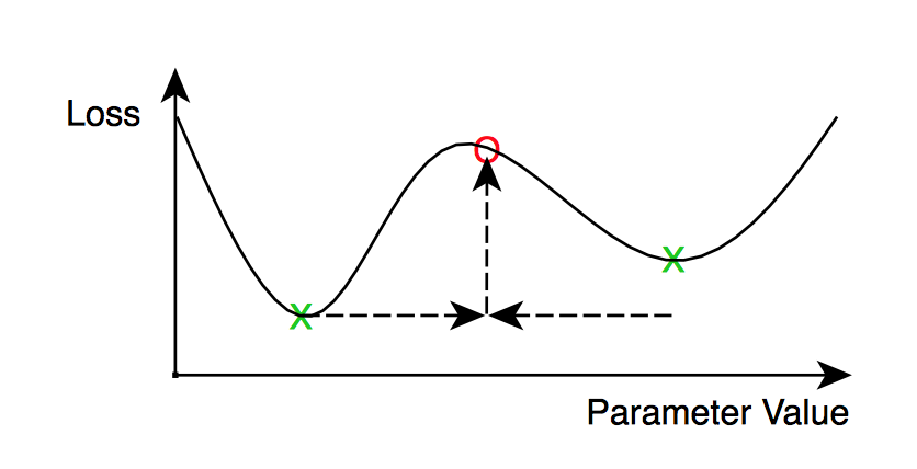
The naive approach is to simply average the parameters after each iteration. While this can work, we are likely to find that the overhead of doing so to be impractically high; network communication and synchronization costs may overwhelm the benefit obtained from the extra machines. Consequently, parameter averaging is generally implemented with an averaging period (in terms of number of minibatches per worker) greater than 1. However, if we average too infrequently, the local parameters in each worker may diverge too much, resulting in a poor model after averaging. The intuition here is that the average of N different local minima are not guaranteed to be a local minima:
:smile: :smile:What averaging period is too high?
This question hasn’t been conclusively answered yet, and is made more complicated by the interaction with other hyperparameters, such as the learning rate, minibatch size and number of workers. Some preliminary research on the subject (such as [8]) suggests that averaging periods on the order of once in every 10 to 20 minibatches (per worker) can still perform acceptably well. Model accuracy is of course reduced as the averaging period is increased.
An additional complication related to optimization methods such as adagrad, momentum and RMSProp. These optimation methods (known as ’updaters’ in Deeplearning4j) have been shown to significantly improve the convergence properties during neural network training.
However, these updaters have internal state (typically 1 or 2 state values per network parameter) - should we average this state also? Averaging the internal updater state should result in faster convergence in each worker, at the cost of doubling - or more - the total size of the network transfers. Some work has also looked at applying similar ‘updater’ mechanisms at the level of the parameter server, and not just in each worker ([1]).
Asynchronous Stochastic Gradient Descent
A conceptually similar approach to parameter averaging is what we might call ‘update based’ data parallelism. The primary difference between the two is that instead of transferring parameters from the workers to the parameter server, we will transfer the updates (i.e., gradients post learning rate and momentum, etc.) instead. This gives an update of the form:
where $\lambda$ is a scaling factor (analogous to a learning rate hyperparameter).
Architecturally, this looks similar to parameter averaging:
Readers familiar with the mathematics of training neural networks may have noticed an immediate similarity here between parameter averaging and the update-based approach. If we again define our loss function as $L$, then parameter vector $W$ at iteration i + 1 for simple SGD training with learning rate $α$ is obtained by: $W_{i+1,j} = W_{i} - \alpha \nabla L_j$ with $\nabla L = \left(\frac{\partial L}{\partial w_1},\ldots,\frac{\partial L}{\partial w_n}\right)$ for $n$ parameters.
Now, if we take the weight update rule shown above, and let $\lambda=\frac{1}{n}$ for $n$ executors, and note that (again using SGD only with learning rate $\alpha$, for brevity)) the update is $\Delta W_{i,j} = \alpha \nabla L_j$, then we have:
Consequently, there is an equivalence between parameter averaging and update-based data parallelism, when parameters are updated synchronously (this last part is key). This equivalence also holds for multiple averaging steps and other updaters (not just simple SGD).
Update-based data parallelism becomes more interesting (and arguably more useful) when we relax the synchronous update requirement. That is, by allowing the updates $∆Wi,j$ to be applied to the parameter vector as soon as they are computed (instead of waiting for $N ≥ 1$ iterations by all workers), we obtain asynchronous stochastic gradient descent algorithm. Async SGD has two main benefits:
-
First, we can potentially gain higher throughput in our distributed system: workers can spend more time performing useful computations, instead of waiting around for the parameter averaging step to be completed.
-
Second, workers can potentially incorporate information (parameter updates) from other workers sooner than when using synchronous (every $N$ steps) updating.
These benefits are not without cost, however. By introducing asynchronous updates to the parameter vector, we introduce a new problem, known as the stale gradient problem. The stale gradient problem is quite simple: the calculation of gradients (updates) takes time. By the time a worker has finished these calculations and applies the results to the global parameter vector, the parameters may have been updated a number of times. This problem is illustrated in the figure below.
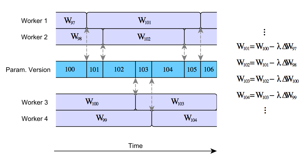
A naive implementation of asynchronous SGD can result is very high staleness values for the gradients. For example, Gupta et al. 2015 [3] show that the average gradient staleness is equal to the number of executors. For $N$ executors, this means that the gradients will be on average N steps out of date by the time they are applied to the global parameter vector. This has real-world consequences: high gradient staleness can slow network convergence significantly, and even stop some configurations from converging at all. Earlier async SGD implementations (such as Google’s DistBelief system [2]) did not account for this effect, and hence learning was considerably less efficient than it otherwise could have been.
Most variants of asynchronous stochastic gradient descent maintain the same basic approach, but apply a variety of strategies to minimize the impact of the stale gradients, whilst attempting to maintaining high cluster utilization. It should be noted that parameter averaging is not subject to the stale gradient problem due to the synchronous nature of the algorithm.
Some approaches to dealing with stale gradients include:
-
Scaling the value λ separately for each update $∆Wi,j$ based on the staleness of the gradients
-
Implementing ‘soft’ synchronization protocols ([9])
-
Use synchronization to bound staleness. For example, the system of [4] delays faster workers when necessary, to ensure that the maximum staleness is below some threshold
All of these approaches have been shown to improve convergence over the naive asynchronous SGD algorithm. Of note especially are the first two: scaling updates based on staleness (stale gradients have a smaller impact on the parameter vector), and soft synchronization. Soft synchronization ([9]) is quite simple: instead of updating the global parameter vector immediately, the parameter server waits to collect some number s of updates $∆Wj$ from any of the n learners (where 1 ≤ s ≤ n). Parameters are then updated according to:
where $ \lambda\left(\Delta W_j\right)$ is a scalar staleness-dependent scaling factor;
[9] propose $ \lambda\left(x\right)=\frac{\lambda_0}{\tau} $ where $ \tau\geq1 $ is an integer based on the staleness of the parameters, though other approaches are possible (see for example [6]). The combination of softsync and staleness–dependent scaling performs better than either does alone.
Note that by setting $s = 1$ and $λ(·) = constant$ we obtain the nave async SGD algorithm (as per [2]); similarly, by s = n we obtain an algorithm similar (but not identical) to synchronous parameter averaging.
Decentralized Asychronous Stochastic Gradient Descent
One of the more interesting alternative architectures for performing distributed training of neural net- works was proposed by [7]. I’ll refer to this approach as decentralized asychronous stochastic gradient descent (though the author does not use this terminology). This paper is interesting for two primary reasons:
- No centralized parameter server is present in the system (instead, peer to peer communication is used to transmit model updates between workers).
- Updates are heavily compressed, resulting in the size of network communications being reduced by some 3 orders of magnitude.
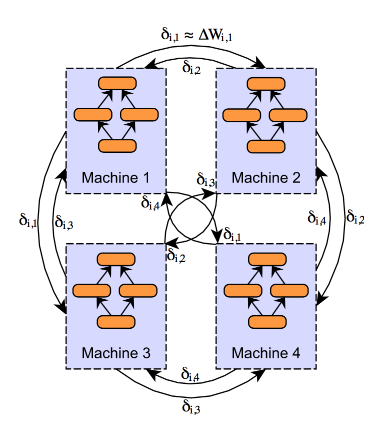
In a standard data parallel implementation (using either parameter averaging or async SGD), the size of the network transfers are equal to the parameter vector size (as we are transferring either copies of the parameter vector, or one gradient value per parameter). While the idea of compressing parameters or updates isn’t exactly new, the implementation goes a way beyond other simple compression mechanisms (such as applying a compression codec or converting to 16-bit floating point representation).
The neat thing about this design is that update vectors $δi,j$ are:
-
Sparse: only some of the gradients are communicated in each vector δi,j (the remainder are assumed to be 0) - sparse entries are encoded using an integer index
-
Quantized to a single bit: each element of the sparse update vector takes value +τ or −τ. This value of τ is the same for all elements of the vector, hence only a single bit is required to differentiate between the two options
-
Integer indexes (used to identify the entries in the sparse array) are optionally compressed using entropy coding to further reduce update sizes (the author quotes a further 3x reduction at the cost of additional computation, though the benefit may not be worth the additional cost)
Furthermore, to account for the fact that the compression method is very lossy, the difference between the original update vector $\Delta W_{i,j}$ and the compressed/quantized update vector $\delta_{i,j}$ is stored in what is known as a residual vector, (r_j) on each executor j, instead of simply being discarded. The residual vector is added to the original update: i.e., we quantize and transmit a compressed version of $\Delta W_{i,j} + r_j$ at each step, updating rj as appropriate. The net effect is that the full information from the original update vector $\Delta W_{i,j}$ is merely delayed, not lost. Put another way, large updates (per parameter) are dynamically transmitted at a higher rate than small updates.
Two questions arise here: (a) how much does this help to reduce network transfers, and (b) how does this impact accuracy? The answers are a lot and less than you might expect.
Take for example a model with 14.6 million parameters, as reported in Strom’s paper:
| Compression | Update Size | Reduction |
|---|---|---|
| None (32-bit floating point) | 58.4 MB | - |
| 16-bit floating point | 29.2 MB | 50% |
| Quantized, $\tau=2$ | 0.21 MB | 99.6% |
Larger values of τ can be used, and result in greater compression (for example, τ = 15 is reported to re- sult in an update size of only 4.5 KB per minibatch!) but model accuracy noticeably suffers as τ increases.
As impressive as the results are, there appear to be three main downsides of this approach.
-
Strom reports that convergence can suffer in the early stages of training (using fewer compute nodes for a fraction of an epoch seems to help)
-
Compression and quantization is not free: these processes result in extra computation time per minibatch, and a small amount of memory overhead per executor
-
The process introduces two additional hyperparameters to consider: the value for τ and whether to use entropy coding for the updates or not (though notably both parameter averaging and async SGD also introduce additional hyperparameters)
Finally, there is not (to the author’s knowledge) any experimental comparisons of asychronous SGD and decentralized async SGD.
Distributed Neural Network Training: Which Approach is Best?
We’ve seen that there are multiple approaches to training distributed neural networks, with a number variants of each type. So which one should we prefer in practice? Unfortunately, there isn’t a simple answer to this question. For one thing, we could define different approaches as best, according to any of the following criteria:
- Fastest training speed (highest number of training examples per second, or lowest time per epoch)
- Maximum attainable accuracy as nepochs $→ ∞$
- Maximum attainable accuracy for a given amount of wall clock time
- Maximum attainable accuracy for a given number of epochs
Furthermore, the answers to these questions will likely depend on a number of factors, such as the type and size of neural network, cluster hardware, use of features such as compression, as well as the specific implementation and configuration of the training method.

That said, there seem to be some conclusions we can draw from the research:
Synchronous parameter averaging (or equivalently, synchronous update-based) approaches win out in terms of accuracy per epoch, and the overall attainable accuracy, especially with small averaging periods. See for example the ‘hardsync’ results in [9], or the fact that synchronous averaging with N = 1 averaging period most closely approximates single machine training. However, the additional synchronization costs mean that this approach is necessarily slower per epoch; that said, fast network interconnects such as InfiniBand can go a long way to keeping synchronous approaches competitive (see for example [5]). However, even on commodity hardware, we see good cluster utilization in practice with DL4J’s synchronous parameter averaging implementation. Adding compression should further help to reduce network communication overheads. Perhaps the greatest issue with parameter averaging (and synchronous approaches in general) is the so-called ‘last executor’ effect: that is, synchronous systems have to wait on the slowest executor before completing each iteration. Consequently, synchronous systems are less viable as the total number of workers increases.
Asynchronous stochastic gradient descent is a good option for training and has been shown to work well in practice, as long as gradient staleness is appropriately handled. Some implementations (such as softsync approach described earlier) can be viewed as spanning a continuum between nave asynchronous SGD and synchronous implementations, depending on the hyperparameters used.
Async SGD implementations with a centralized parameter server may introduce a communication bottleneck (by comparison, synchronous approaches may utilize tree-reduce or similar algorithms, avoiding some of this communication bottleneck). Utilizing $N$ parameter servers, each handling an equal fraction of the total parameters is a conceptually straightforward solution to this problem.
Finally, decentralized asynchronous stochastic gradient descent is a promising idea, though further research is required before we can conclusively recommend this over ‘standard’ async SGD. Furthermore, many of the ideas (compression, quantization, etc.) from [7] could be adapted to async SGD implementations that utilize a more traditional parameter server design.
When to Use Distributed Deep Learning
Performing deep learning in a distributed manner isn’t always the best option, for every use case.
Distributed training isn’t free - distributed systems necessarily have an overhead compared to training on a single machine, due to things like synchonization and network transfers of data and parameters. For distributed training to be worthwhile, we need the computational benefit of the additional machines to outweigh these overheads. Furthermore, setup time (i.e., preparing and loading training data) and hyperparameter tuning can be more complex in distributed systems. Consequently, our advice is simple: continue to train your networks on a single machine, until the training time becomes prohibitive.
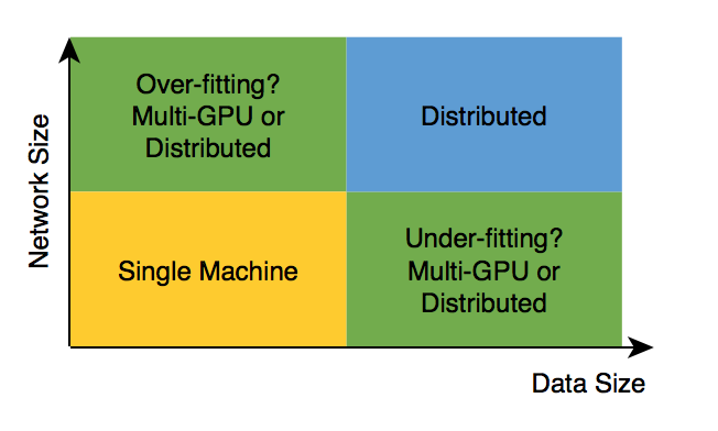
Network training times can become prohibitive for two reasons: either network size is large (costly per iteration), or the amount of data is large. Often, these go hand in hand; in fact, a mismatch between the two (large network, small data; small network, lots of data) may lead to underfitting or overfitting - both can lead to poor generalization of the final trained model.
In some cases, multi-GPU systems should be considered before (for example, Deeplearning4j’s Parallel-Wrapper implementation allows for easy data parallel training of networks on a single machine). Model parallelism using multi-GPU systems may also be viable for large networks.
Another perspective is to consider the ratio of network transfers to computation. Distributed training tends to be more efficient when the ratio of transfers to computation is low. Small and shallow networks are not good candidates for distributed training as they don’t have much computation per iteration. Networks with parameter sharing (such as CNNs and RNN) tend to be good candidates for distributed training: the amount of computation per parameter is much higher than, for example, a multi-layer perceptron or autoencoder architecture.
References
[1] Kai Chen and Qiang Huo. Scalable training of deep learning machines by incremental block training with intra-block parallel optimization and blockwise model-update filtering. In 2016 IEEE International Conference on Acoustics, Speech and Signal Processing (ICASSP), pages 5880–5884. IEEE, 2016.
[2] Jeffrey Dean, Greg Corrado, Rajat Monga, Kai Chen, Matthieu Devin, Mark Mao, Andrew Senior, Paul Tucker, Ke Yang, Quoc V Le, et al. Large scale distributed deep networks. In Advances in Neural Information Processing Systems, pages 1223–1231, 2012.
[3] Suyog Gupta, Wei Zhang, and Josh Milthrope. Model accuracy and runtime tradeoff in distributed deep learning. arXiv preprint arXiv:1509.04210, 2015.
[4] Qirong Ho, James Cipar, Henggang Cui, Seunghak Lee, Jin Kyu Kim, Phillip B. Gibbons, Garth A Gibson, Greg Ganger, and Eric P Xing. More effective distributed ml via a stale synchronous parallel parameter server. In C. J. C. Burges, L. Bottou, M. Welling, Z. Ghahramani, and K. Q. Weinberger, editors, Advances in Neural Information Processing Systems 26, pages 1223–1231. Curran Associates, Inc., 2013.
[5] Forrest N Iandola, Khalid Ashraf, Mattthew W Moskewicz, and Kurt Keutzer. Firecaffe: near-linear acceleration of deep neural network training on compute clusters. arXiv preprint arXiv:1511.00175, 2015.
[6] Augustus Odena. Faster asynchronous sgd. arXiv preprint arXiv:1601.04033, 2016.
[7] Nikko Strom. Scalable distributed dnn training using commodity gpu cloud computing. In Sixteenth Annual Conference of the International Speech Communication Association, 2015. http://nikkostrom.com/publications/interspeech2015/strom_interspeech2015.pdf.
[8] Hang Su and Haoyu Chen. Experiments on parallel training of deep neural network using model averaging. arXiv preprint arXiv:1507.01239, 2015.
[9] Wei Zhang, Suyog Gupta, Xiangru Lian, and Ji Liu. Staleness-aware async-sgd for distributed deep learning. IJCAI, 2016.