Bptt反向传播算法 In Rnn

In this part we’ll give a brief overview of BPTT and explain how it differs from traditional backpropagation. We will then try to understand the vanishing gradient problem which has led to the development of LSTMs and GRUs, two of the currently most popular and powerful models used in NLP (and other areas). 我的参考／学习资料

其他资料：

知乎 - 有哪些LSTM(Long Short Term Memory)和RNN(Recurrent)网络的教程

Table fo Contents

[toc]

Preliminary

If you are not familiar with how partial differentiation and basic backpropagation works. you can find a great tutorial here CS231n Convolutional Neural Networks for Visual Recognition - ptimizaton. Yes, I used this tutorial before.

Backpropagation Through Time (BPTT)

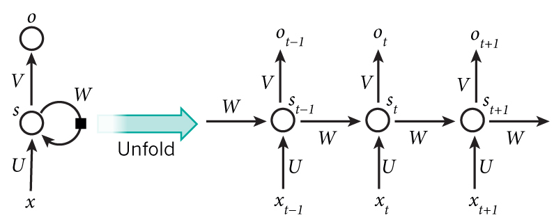
Let’s quickly recap the basic equations of our RNN.

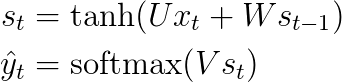
We also defined our loss, or error, to be the cross entropy loss, given by:

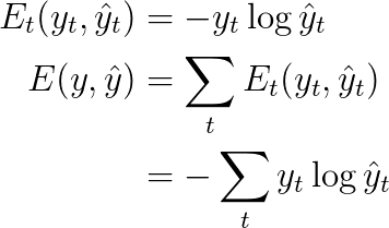
Here, $y_t$ is the correct word at time step $t$, and $\hat{y}_t$ is our prediction. We typically treat the full sequence (sentence) as one training example, so the total error is just the sum of the errors at each time step (word).

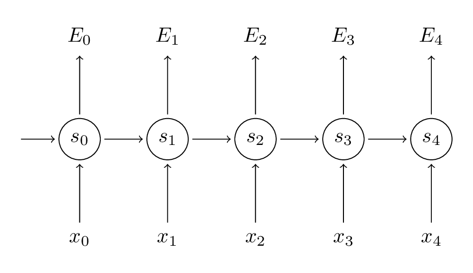
Remember that our goal is to calculate the gradients of the error with respect to our parameters $U, V$ and $W$ and then learn good parameters using Stochastic Gradient Descent. Just like we sum up the errors, we also sum up the gradients at each time step for one training example:

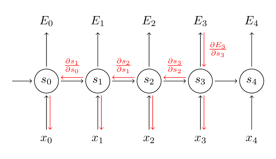
$\frac{\partial E}{\partial W} = \sum\limits_{t} \frac{\partial E_t}{\partial W}.$

To calculate these gradients we use the chain rule of differentiation. That’s the backpropagation algorithm when applied backwards starting from the error. For the rest of this post we’ll use $E_3$ as an example, just to have concrete numbers to work with.

$\begin{aligned} \frac{\partial E_3}{\partial V} &=\frac{\partial E_3}{\partial \hat{y}_3}\frac{\partial\hat{y}_3}{\partial V}\\ &=\frac{\partial E_3}{\partial \hat{y}_3}\frac{\partial\hat{y}_3}{\partial z_3}\frac{\partial z_3}{\partial V}\\ &=(\hat{y}_3 - y_3) \otimes s_3 \\ \end{aligned}$

In the above, $z_3 =Vs_3$, and $\otimes$ is the outer product of two vectors. Don’t worry if you don’t follow the above, I skipped several steps and you can try calculating these derivatives yourself (good exercise!). The point I’m trying to get across is that $\frac{\partial E_3}{\partial V}$ only depends on the values at the current time step, $\hat{y}_3, y_3, s_3$ . If you have these, calculating the gradient for $V$ a simple matrix multiplication.

But the story is different for $\frac{\partial E_3}{\partial W} $(and for $U$). To see why, we write out the chain rule, just as above:

$\begin{aligned} \frac{\partial E_3}{\partial W} &= \frac{\partial E_3}{\partial \hat{y}_3}\frac{\partial\hat{y}_3}{\partial s_3}\frac{\partial s_3}{\partial W}\\ \end{aligned}$

Now, note that $s_3 = \tanh(Ux_t + Ws_2)$ depends on $s_2$, which depends on $W$ and $s_1$, and so on. So if we take the derivative with respect to $W$ we can’t simply treat $s_2$ as a constant! We need to apply the chain rule again and what we really have is this:

$\begin{aligned} \frac{\partial E_3}{\partial W} &= \sum\limits_{k=0}^{3} \frac{\partial E_3}{\partial \hat{y}_3}\frac{\partial\hat{y}_3}{\partial s_3}\frac{\partial s_3}{\partial s_k}\frac{\partial s_k}{\partial W}\\ \end{aligned}$

We sum up the contributions of each time step to the gradient. In other words, because $W$ is used in every step up to the output we care about, we need to backpropagate gradients from $t=3$ through the network all the way to t=0:

Note that this is exactly the same as the standard backpropagation algorithm that we use in deep Feedforward Neural Networks. The key difference is that we sum up the gradients for W at each time step. In a traditional NN we don’t share parameters across layers, so we don’t need to sum anything. But in my opinion BPTT is just a fancy name for standard backpropagation on an unrolled RNN. Just like with Backpropagation you could define a delta vector that you pass backwards, e.g.: $\delta_2^{(3)} = \frac{\partial E_3}{\partial z_2} =\frac{\partial E_3}{\partial s_3}\frac{\partial s_3}{\partial s_2}\frac{\partial s_2}{\partial z_2}$ with $z_2 = Ux_2+ Ws_1$. Then the same equations will apply.

In code, a naive implementation of BPTT looks something like this:

def bptt(self, x, y):
    T = len(y)
    # Perform forward propagation
    o, s = self.forward_propagation(x)
    # We accumulate the gradients in these variables
    dLdU = np.zeros(self.U.shape)
    dLdV = np.zeros(self.V.shape)
    dLdW = np.zeros(self.W.shape)
    delta_o = o
    delta_o[np.arange(len(y)), y] -= 1.
    # For each output backwards...
    for t in np.arange(T)[::-1]:
        dLdV += np.outer(delta_o[t], s[t].T)
        # Initial delta calculation: dL/dz
        delta_t = self.V.T.dot(delta_o[t]) * (1 - (s[t] ** 2))
        # Backpropagation through time (for at most self.bptt_truncate steps)
        for bptt_step in np.arange(max(0, t-self.bptt_truncate), t+1)[::-1]:
            # print "Backpropagation step t=%d bptt step=%d " % (t, bptt_step)
            # Add to gradients at each previous step
            dLdW += np.outer(delta_t, s[bptt_step-1])
            dLdU[:,x[bptt_step]] += delta_t
            # Update delta for next step dL/dz at t-1
            delta_t = self.W.T.dot(delta_t) * (1 - s[bptt_step-1] ** 2)
    return [dLdU, dLdV, dLdW]

This should also give you an idea of why standard RNNs are hard to train: Sequences (sentences) can be quite long, perhaps 20 words or more, and thus you need to back-propagate through many layers. In practice many people truncate the backpropagation to a few steps.